MRP norming tutorial
2024-02-18
knitr::opts_chunk$set(
    message = FALSE,
    warning = FALSE,
    include = TRUE,
    error = TRUE,
    fig.width = 8,
    fig.height = 4
)
1 Load dependencies and required datasets
If you don’t have access to the TwinLife data, comment out the “preprocessed TwinLife data” chunk and run the “synthetic TwinLife data” chunk instead. IMPORTANT: If you’re using the synthetic dataset, not all analyses will reproduce those based on the actual data because synthpop does not model interactions between variables.
1.1 Required packages and options
library(tidyverse)
library(ggrepel)
library(kableExtra)
library(brms)
library(tidybayes)
library(marginaleffects)
library(bayesplot)

# depending on the platform on which you want to run the brm you might need this or not. We ran the models on a Linux-operated server, cmdstanr version 0.5.3
options(mc.cores = 4,
        brms.backend = "cmdstanr")

options(scipen = 999,
        digits = 4)

# windowsFonts(Times = windowsFont("Times New Roman"))
theme_set(theme_minimal(base_size = 12, base_family = "Times"))
1.2 Preprocessed TwinLife data
load("data/preprocessed/census.Rda")
load("data/preprocessed/census_marginals.Rda")
load("../unshareable_data/preprocessed/tl.Rda")

# exclude first twins to avoid twin dependency issues and add variable containing the age groups from the manual
tl_no_1st_twins <- tl %>%
 filter(ptyp != 1)
1.3 Synthetic TwinLife data
# load("data/preprocessed/census.Rda")
# load("data/preprocessed/census_marginals.Rda")
# load("data/simulated/synthetic_tl.Rda")

# tl_no_1st_twins <- synthetic_tl
2 Distributional disparities
Before applying MRP to correct estimates (be it for norming or other purposes), it’s worthwhile to check if there are any differences between the sample and the population (on which we have data from the census) with respect to the variables we wish to use for the correction. Here we first look at disparities at the level of marginal distributions (e.g., is the overall proportion of males to females similar in our sample to the population?), then at the joint distribution level (e.g., are female citizens with no migration background, aged 67, who have a general secondary school certificate as well represented in our sample as in the population?).
2.1 Marginal
One plot for age and one for the three other variables.
# Custom sorting function
custom_sort <- function(x) {
  st_categories <- x[startsWith(x, "ST")]
  isced_categories <- x[startsWith(x, "ISCED")]
  other_categories <- x[!startsWith(x, "ST") & !startsWith(x, "ISCED")]

  factor(x, levels = c(sort(st_categories), sort(isced_categories), other_categories))
}

# get the marginal distributions from the census and the TL sample
disparities_plot <- census %>%
  full_join(tl_no_1st_twins %>%
  group_by(age0100, male, educ, mig) %>%
  summarise(sample_n = n()) %>%
  rename(age = "age0100") %>%
  mutate(sample_n = as.numeric(sample_n)), by = c("age", "male", "educ", "mig")) %>%
  mutate(sample_n = replace_na(sample_n, 0)) %>%
  pivot_longer(cols = c(census_n:sample_n), names_to = "source", values_to = "n") %>%
  mutate(age = as.character(age),
         male = as.character(male),
         source = str_sub(source, 1, -3)) %>%
pivot_longer(cols = -c(n, source), names_to = "variable", values_to = "category") %>%
  group_by(source, variable, category) %>%
  summarise(n = sum(n)) %>%
  mutate(percentage = n/sum(n)*100) %>%
  filter(source == "sample") %>%
  bind_rows(census_marginals) %>%
  mutate(category = case_when(
    category == "TRUE" ~ "Male",
    category == "FALSE" ~ "Female",
    TRUE ~ category)) %>%
  mutate(category = custom_sort(category))


# plot age disparities
disparities_plot %>%
  filter(variable == "age") %>%
  ggplot(aes(x = category, y = percentage, group = source, colour = source, label = round(percentage, digits = 1))) +
  geom_line(linewidth = 1) +
  facet_grid(cols = vars(variable), scales = "free", space = 'free', as.table = FALSE,
             labeller = labeller(variable = function(variable) {
               case_when(
                 variable == "age" ~ "Age",
                 TRUE ~ as.character(variable))})) +
  theme(axis.text.x = element_text(angle = 45, hjust = 1),
        legend.position = c(1, 1.08),  #
        legend.justification = c(1, 1),
        legend.background = element_rect(fill = "transparent", color = NA),
        panel.grid.major.y = element_blank(),
        panel.grid.minor.y = element_blank(),
        panel.grid.major.x = element_line(linetype = "dashed", size = 0.3)) +
  labs(x = "Category", y = "Percentage", colour = "", label = "Percentage") +
  scale_colour_manual(values = c("#0072b2", "#e69f00"), labels = function(x) str_to_title(x)) +
  scale_x_discrete(breaks = seq(12, 79, by = 2))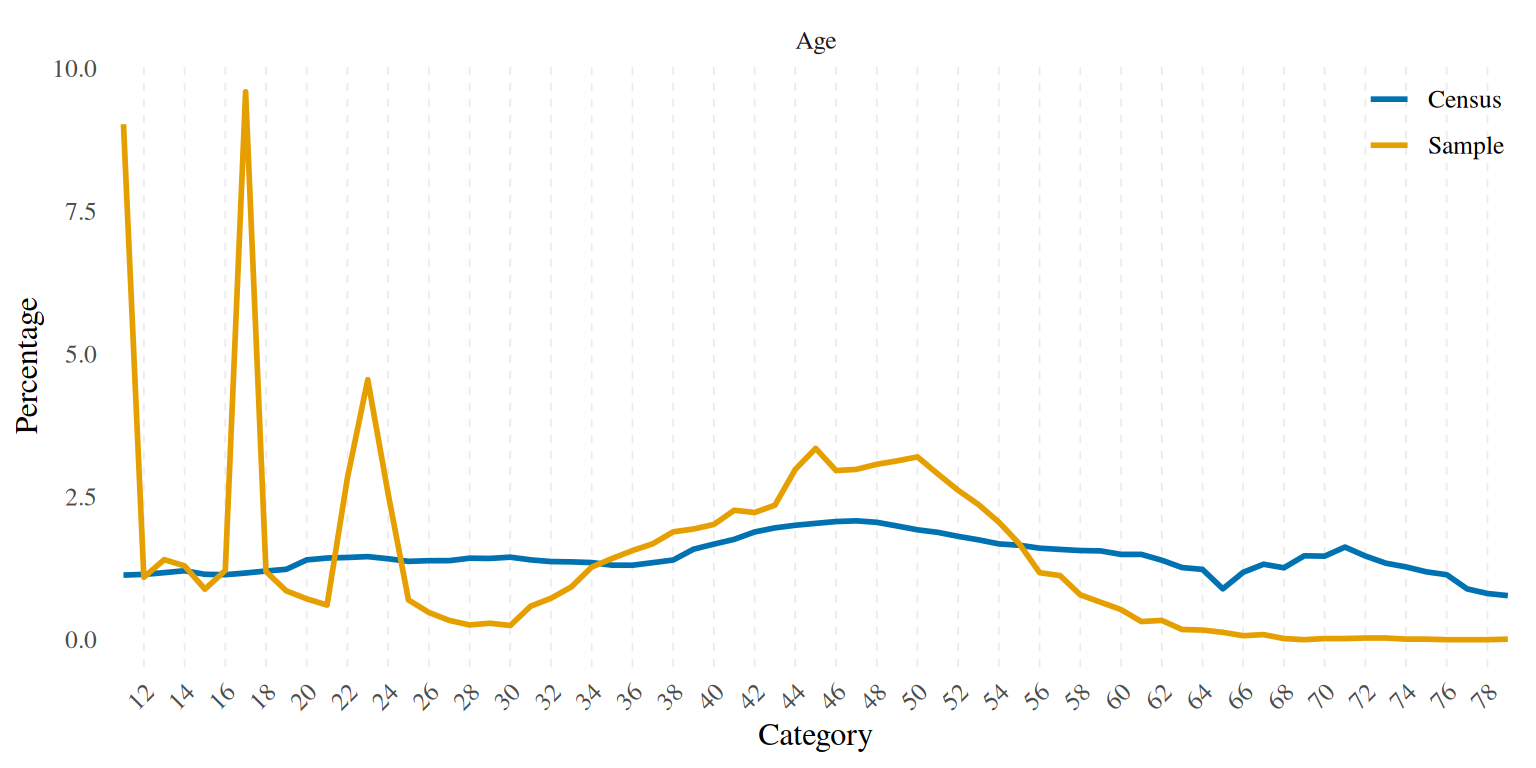
disparities_plot %>%
  filter(variable != "age") %>%
  ggplot(aes(x = category, y = percentage, group = source, colour = source, label = round(percentage, digits = 1))) +
  geom_line(linewidth = 1) +
 # theme_minimal(base_size = 14, base_family = "Times") +
  facet_grid(
    cols = vars(variable),
    scales = "free",
    space = 'free',
    as.table = FALSE,
    labeller = labeller(variable = function(variable) {
      case_when(
        variable == "educ" ~ "School Type / ISCED 1997 Code",
        variable == "male" ~ "Sex",
        variable == "mig" ~ "Migration",
        TRUE ~ as.character(variable))})) +
   theme(axis.text.x = element_text(angle = 45, hjust = 1),
        legend.position = c(1, 1.1),  #
        legend.justification = c(1, 1),
        legend.background = element_rect(fill = "transparent", color = NA),
         panel.grid.major.y = element_blank(),
         panel.grid.minor.y = element_blank(),
         panel.grid.major.x = element_line(linetype = "dashed", size = 0.3)) +
  labs(x = "Category", y = "Percentage", colour = "", label = "Percentage") +
  scale_colour_manual(values = c("#0072b2", "#e69f00"), labels = function(x) str_to_title(x))+
  labs(x = "Category", y = "Percentage", colour = "", label = "Percentage") +
  geom_text_repel(family = "Times", seed = 14, point.padding = 2, direction = "y", hjust = 0)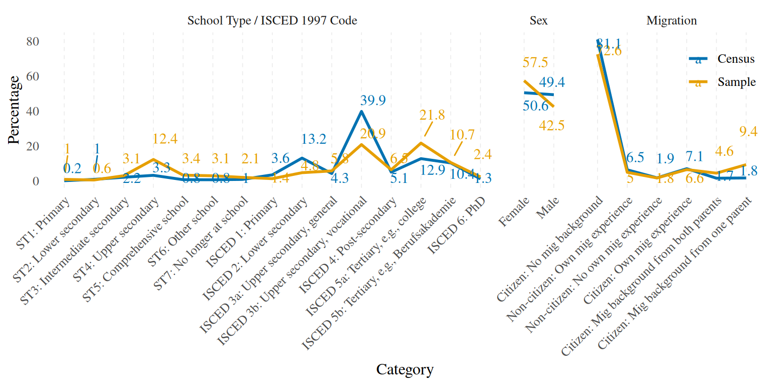
Besides the obvious age disparities due to the cohort design adopted to collect the data for the TwinLife sample, we also see that our sample is “overeducated” in the sense that for example we have too many kids who were going to the Gymnasium (ST4: upper secondary) and too few adults who have something similar to an Ausbildungsabschluss (ISCED 3b: upper secondary, vocational). Migrants and females are also overrepresented in the sample.
2.2 Joint
You can use this interactive table to browse disparities at the level of joint distributions, ordered after magnitude. Note that this table has 6528 rows (number of subgroups/combinations of the 4 variables we use). Most of these subgroups are empty in the sample.
census %>%
  full_join(tl_no_1st_twins %>%
  group_by(age0100, male, educ, mig) %>%
  summarise(sample_n = n()) %>%
  rename(age = "age0100") %>%
  mutate(sample_n = as.numeric(sample_n)), by = c("age", "male", "educ", "mig")) %>%
  # set the subgroups which are empty in the sample to 0 instead of NA
  mutate(sample_n = replace_na(sample_n, 0)) %>%
  group_by(age, male, educ, mig) %>%
  summarise(census_n = sum(census_n),
            sample_n = sum(sample_n)) %>%
  group_by(age) %>%
  mutate(census_percentage = census_n*100/sum(census_n),
         sample_percentage = sample_n*100/sum(sample_n),
         dif_percentage = census_percentage-sample_percentage,
         relative_dif = dif_percentage*census_n/100,
         age = as.integer(age)) %>%
  relocate(census_percentage, .after = "census_n") %>%
  arrange(-relative_dif) %>% DT::datatable() %>%
  DT::formatRound(c('dif_percentage', 'relative_dif', 'census_percentage', 'sample_percentage'), digits = 1)
3 Regularised prediction model
This is the MR part of MRP.
3.1 Fit the model
Terms of this form (1 | variable) represent random
intercepts, (male) was included as a fixed effect to avoid
estimation problems due to the small number of categories,
s(age) is a thin plate spline of age, and
s(age, by = educ) fits a separate spline of age within each
category of educ. We don’t include this latter term in the
\(\sigma\) prediction part of the model
because it is unnecessarily complex given the heterogeneity in the
variance and it leads to a lot of divergent transitions.
3.1.1 On the TwinLife data
brm_age_by_educ <-
  brm(bf(
      cft ~ (1 | mig)  + (male)  + (1 | mig:male) + (1 | mig:educ) + (1 | male:educ) + (1 | mig:educ:male) + s(age, by = educ),
      sigma ~ (1 | mig) + (1 | educ) + (male)  + (1 | mig:male) + (1 | mig:educ) + (1 | male:educ) + (1 | mig:educ:male) + s(age)),
      family = gaussian(),
      chains = 4,
      iter = 5000,
      seed = 810,
      control = list(adapt_delta = 0.99),
      file = "../unshareable_data/brms/brm_age_by_educ_18_delta_99_5000",
      file_refit = "never",
      data = tl_no_1st_twins) %>%
  add_criterion("loo")
3.1.2 On the synthetic data
# brm_age_by_educ <-
#   brm(bf(
#       cft ~ (1 | mig)  + (male)  + (1 | mig:male) + (1 | mig:educ) + (1 | male:educ) + (1 | mig:educ:male) + s(age, by = educ),
#       sigma ~ (1 | mig) + (1 | educ) + (male)  + (1 | mig:male) + (1 | mig:educ) + (1 | male:educ) + (1 | mig:educ:male) + s(age)),
#       family = gaussian(),
#       chains = 4,
#       iter = 5000,
#       seed = 14,
#       control = list(adapt_delta = 0.99),
#       file = "data/brms/brm_age_by_educ_18_delta_99_5000_synth",
#       file_refit = "never",
#       data = tl_no_1st_twins) %>%
#   add_criterion("loo")

# alternatively, load the .rds file for the model we ran on the synthetic data
# brm_age_by_educ <- readRDS("data/brms/brm_age_by_educ_18_delta_99_5000_synth.rds")
3.2 Some model exploration
3.2.1 Summary
brm_age_by_educ## Warning: There were 2 divergent transitions after warmup. Increasing
## adapt_delta above 0.99 may help. See
## http://mc-stan.org/misc/warnings.html#divergent-transitions-after-warmup## Family: gaussian
## Links: mu = identity; sigma = log
## Formula: cft ~ (1 | mig) + (male) + (1 | mig:male) + (1 | mig:educ) + (1 | male:educ) + (1 | mig:educ:male) + s(age, by = educ)
## sigma ~ (1 | mig) + (1 | educ) + (male) + (1 | mig:male) + (1 | mig:educ) + (1 | male:educ) + (1 | mig:educ:male) + s(age)
## Data: tl_no_1st_twins (Number of observations: 10059)
## Draws: 4 chains, each with iter = 5000; warmup = 2500; thin = 1;
## total post-warmup draws = 10000
##
## Smooth Terms:
## Estimate Est.Error l-95% CI
## sds(sageeducISCED3b:Uppersecondaryvocational_1) 10.54 4.39 4.62
## sds(sageeducISCED1:Primary_1) 21.34 15.41 2.21
## sds(sageeducISCED2:Lowersecondary_1) 15.50 8.69 2.99
## sds(sageeducISCED3a:Uppersecondarygeneral_1) 12.29 10.27 0.43
## sds(sageeducISCED4:PostMsecondary_1) 9.90 5.18 2.71
## sds(sageeducISCED5a:Tertiarye.g.college_1) 11.41 6.57 3.87
## sds(sageeducISCED5b:Tertiarye.g.Berufsakademie_1) 10.67 4.53 4.74
## sds(sageeducISCED6:PhD_1) 12.87 7.81 1.35
## sds(sageeducST1:Primary_1) 9.80 10.82 0.30
## sds(sageeducST2:Lowersecondary_1) 12.57 11.58 0.42
## sds(sageeducST3:Intermediatesecondary_1) 29.63 20.89 8.77
## sds(sageeducST4:Uppersecondary_1) 36.37 18.50 16.00
## sds(sageeducST5:Comprehensiveschool_1) 37.65 24.82 14.80
## sds(sageeducST6:Otherschool_1) 30.13 16.43 11.34
## sds(sageeducST7:Nolongeratschool_1) 16.09 18.84 0.39
## sds(sigma_sage_1) 0.22 0.21 0.01
## u-95% CI Rhat Bulk_ESS
## sds(sageeducISCED3b:Uppersecondaryvocational_1) 21.38 1.00 2711
## sds(sageeducISCED1:Primary_1) 60.78 1.00 986
## sds(sageeducISCED2:Lowersecondary_1) 37.14 1.00 1513
## sds(sageeducISCED3a:Uppersecondarygeneral_1) 38.03 1.00 1754
## sds(sageeducISCED4:PostMsecondary_1) 22.42 1.00 2954
## sds(sageeducISCED5a:Tertiarye.g.college_1) 28.69 1.00 1973
## sds(sageeducISCED5b:Tertiarye.g.Berufsakademie_1) 21.80 1.00 3578
## sds(sageeducISCED6:PhD_1) 31.82 1.00 1559
## sds(sageeducST1:Primary_1) 38.46 1.00 2726
## sds(sageeducST2:Lowersecondary_1) 40.56 1.00 2367
## sds(sageeducST3:Intermediatesecondary_1) 85.67 1.00 1577
## sds(sageeducST4:Uppersecondary_1) 85.05 1.00 3546
## sds(sageeducST5:Comprehensiveschool_1) 100.68 1.00 1785
## sds(sageeducST6:Otherschool_1) 72.64 1.00 1927
## sds(sageeducST7:Nolongeratschool_1) 69.60 1.01 1166
## sds(sigma_sage_1) 0.76 1.00 1897
## Tail_ESS
## sds(sageeducISCED3b:Uppersecondaryvocational_1) 3510
## sds(sageeducISCED1:Primary_1) 1460
## sds(sageeducISCED2:Lowersecondary_1) 1633
## sds(sageeducISCED3a:Uppersecondarygeneral_1) 2595
## sds(sageeducISCED4:PostMsecondary_1) 2550
## sds(sageeducISCED5a:Tertiarye.g.college_1) 2467
## sds(sageeducISCED5b:Tertiarye.g.Berufsakademie_1) 5688
## sds(sageeducISCED6:PhD_1) 1074
## sds(sageeducST1:Primary_1) 3477
## sds(sageeducST2:Lowersecondary_1) 3173
## sds(sageeducST3:Intermediatesecondary_1) 1556
## sds(sageeducST4:Uppersecondary_1) 3611
## sds(sageeducST5:Comprehensiveschool_1) 1274
## sds(sageeducST6:Otherschool_1) 1784
## sds(sageeducST7:Nolongeratschool_1) 982
## sds(sigma_sage_1) 2317
##
## Group-Level Effects:
## ~male:educ (Number of levels: 30)
## Estimate Est.Error l-95% CI u-95% CI Rhat Bulk_ESS Tail_ESS
## sd(Intercept) 3.25 0.85 1.96 5.26 1.00 931 1554
## sd(sigma_Intercept) 0.02 0.01 0.00 0.05 1.00 2438 3885
##
## ~mig (Number of levels: 6)
## Estimate Est.Error l-95% CI u-95% CI Rhat Bulk_ESS Tail_ESS
## sd(Intercept) 2.87 1.26 1.38 6.05 1.00 2342 4242
## sd(sigma_Intercept) 0.06 0.05 0.00 0.18 1.00 1311 1893
##
## ~mig:educ (Number of levels: 89)
## Estimate Est.Error l-95% CI u-95% CI Rhat Bulk_ESS Tail_ESS
## sd(Intercept) 0.62 0.27 0.08 1.16 1.00 1124 919
## sd(sigma_Intercept) 0.09 0.02 0.05 0.13 1.00 1621 1637
##
## ~mig:educ:male (Number of levels: 175)
## Estimate Est.Error l-95% CI u-95% CI Rhat Bulk_ESS Tail_ESS
## sd(Intercept) 0.45 0.25 0.03 0.95 1.00 1021 2461
## sd(sigma_Intercept) 0.02 0.02 0.00 0.06 1.00 1645 2079
##
## ~mig:male (Number of levels: 12)
## Estimate Est.Error l-95% CI u-95% CI Rhat Bulk_ESS Tail_ESS
## sd(Intercept) 0.29 0.30 0.01 1.11 1.00 2925 3699
## sd(sigma_Intercept) 0.03 0.02 0.00 0.09 1.00 2328 3200
##
## ~educ (Number of levels: 15)
## Estimate Est.Error l-95% CI u-95% CI Rhat Bulk_ESS Tail_ESS
## sd(sigma_Intercept) 0.05 0.03 0.00 0.12 1.00 1143 1311
##
## Population-Level Effects:
## Estimate Est.Error l-95% CI
## Intercept 36.54 1.73 33.21
## sigma_Intercept 1.96 0.04 1.87
## maleTRUE 1.02 1.24 -1.45
## sigma_maleTRUE 0.01 0.03 -0.06
## sage:educISCED3b:Uppersecondaryvocational_1 -40.11 24.82 -94.69
## sage:educISCED1:Primary_1 -90.52 79.46 -296.65
## sage:educISCED2:Lowersecondary_1 -56.11 45.94 -168.94
## sage:educISCED3a:Uppersecondarygeneral_1 -36.68 38.86 -140.39
## sage:educISCED4:PostMsecondary_1 -23.34 25.53 -78.79
## sage:educISCED5a:Tertiarye.g.college_1 -9.77 30.89 -54.58
## sage:educISCED5b:Tertiarye.g.Berufsakademie_1 -20.98 25.23 -72.52
## sage:educISCED6:PhD_1 1.14 37.34 -58.33
## sage:educST1:Primary_1 36.89 36.17 -37.55
## sage:educST2:Lowersecondary_1 64.91 45.10 -26.98
## sage:educST3:Intermediatesecondary_1 66.80 100.64 -111.45
## sage:educST4:Uppersecondary_1 46.65 103.78 -155.86
## sage:educST5:Comprehensiveschool_1 36.88 137.36 -223.34
## sage:educST6:Otherschool_1 50.42 92.40 -145.93
## sage:educST7:Nolongeratschool_1 31.07 71.77 -86.37
## sigma_sage_1 0.11 0.55 -0.96
## u-95% CI Rhat Bulk_ESS Tail_ESS
## Intercept 40.16 1.00 1388 2163
## sigma_Intercept 2.05 1.01 2238 2865
## maleTRUE 3.45 1.00 1834 2923
## sigma_maleTRUE 0.07 1.00 3952 4500
## sage:educISCED3b:Uppersecondaryvocational_1 3.91 1.00 1672 1974
## sage:educISCED1:Primary_1 7.98 1.00 769 718
## sage:educISCED2:Lowersecondary_1 10.99 1.00 1417 997
## sage:educISCED3a:Uppersecondarygeneral_1 19.26 1.00 1954 2204
## sage:educISCED4:PostMsecondary_1 25.27 1.00 3075 3782
## sage:educISCED5a:Tertiarye.g.college_1 68.65 1.00 1949 1786
## sage:educISCED5b:Tertiarye.g.Berufsakademie_1 29.44 1.00 3284 4519
## sage:educISCED6:PhD_1 92.13 1.00 1766 2703
## sage:educST1:Primary_1 109.65 1.00 1962 2178
## sage:educST2:Lowersecondary_1 152.11 1.00 1290 1420
## sage:educST3:Intermediatesecondary_1 289.81 1.00 1242 847
## sage:educST4:Uppersecondary_1 264.86 1.00 2016 3056
## sage:educST5:Comprehensiveschool_1 245.72 1.00 1045 933
## sage:educST6:Otherschool_1 225.97 1.01 1018 470
## sage:educST7:Nolongeratschool_1 214.00 1.01 486 602
## sigma_sage_1 1.34 1.00 2216 1857
##
## Draws were sampled using sample(hmc). For each parameter, Bulk_ESS
## and Tail_ESS are effective sample size measures, and Rhat is the potential
## scale reduction factor on split chains (at convergence, Rhat = 1).Despite the boosted adapt_delta, we still had 2
divergent transitions. However, we reran this model multiple times with
different adapt_delta and sometimes had up to 100 divergent
transitions without affecting the fit of the model. We can conclude that
the 4 chains converged since the Rhats are consistently
\(<1.01\). We see that the sd
Estimates of the random intercepts for \(\sigma\) are pretty small so we don’t
expect large variations in the residual variance depending on the
predictors. Larger sds can be observed for predicting \mu
(i.e., the actual CFT 20-R Scores). Males scored on average 0.96 on CFT
20-R than females. Spline related estimates are much harder to interpret
so instead we’ll at some plots.
3.2.2 Check general model fit
pp_check(brm_age_by_educ) 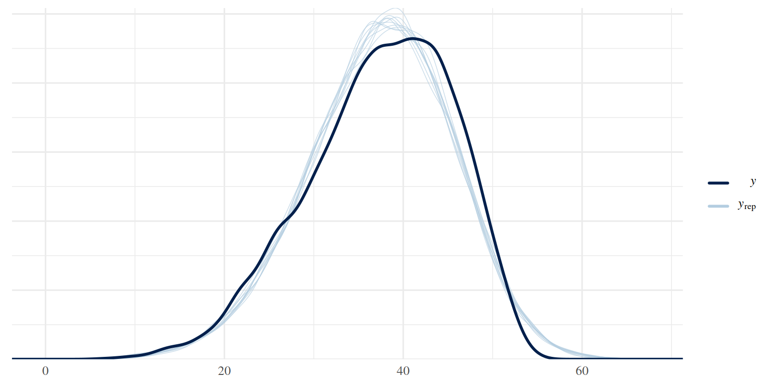
y <- tl_no_1st_twins$cft
yrep <- posterior_predict(brm_age_by_educ, newdata = tl_no_1st_twins, ndraws = 1000)
ppc_pit_ecdf(y, yrep, prob = 0.99, plot_diff = TRUE)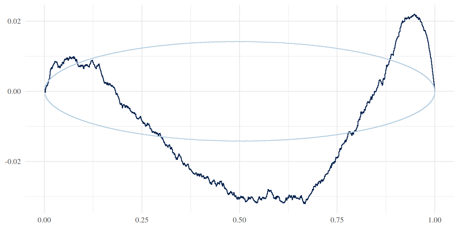
ppc_pit_ecdf(y, yrep, prob = 0.99, plot_diff = FALSE)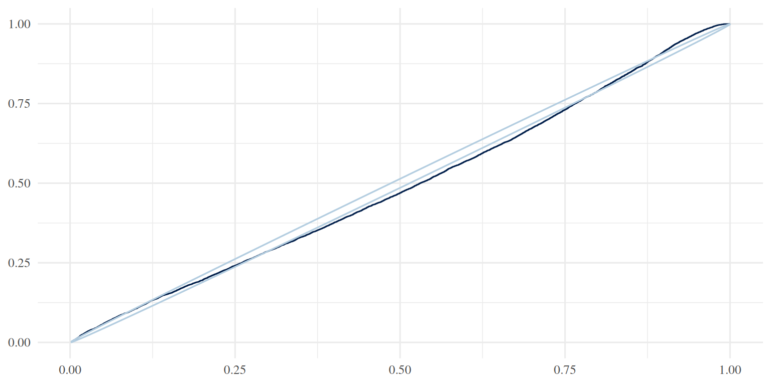
3.2.3 Check fit within age groups
t <- tl_no_1st_twins %>%
 filter(!is.na(age_group))

yrep <- posterior_predict(brm_age_by_educ, newdata = t, ndraws = 1000)


p <- ppc_pit_ecdf_grouped(t$cft, yrep, group = as.factor(t$age_group), prob = 0.99, plot_diff = F)

p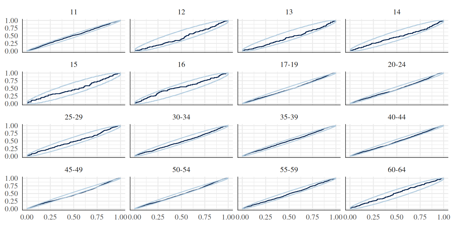
3.2.4 R2
loo_R2(brm_age_by_educ)## Estimate Est.Error Q2.5 Q97.5
## R2 0.3049 0.007551 0.2899 0.31963.2.5 Prediction plots for education and migration background
plot_predictions(brm_age_by_educ,  condition = c("educ"), allow_new_levels = T) +
  labs(x = "Education", y = "CFT 20-R Score") +
theme(axis.text.x = element_text(angle = 60, hjust = 1),
plot.margin = margin(0.8, 2, 0.8, 2, "cm")) 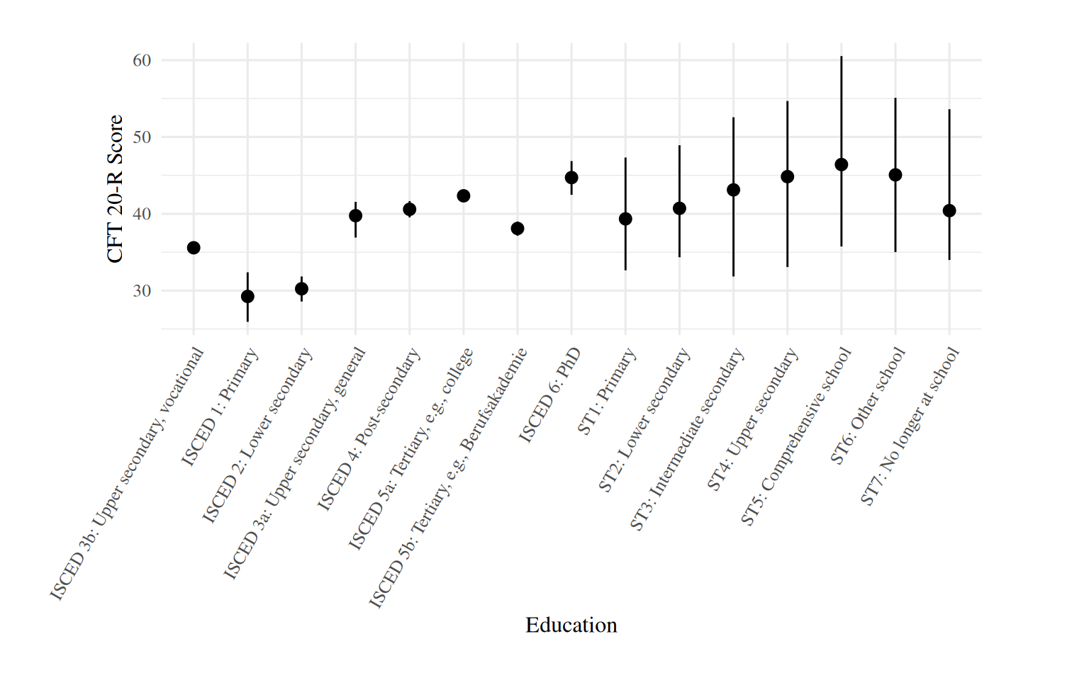
We see that means differ considerably across categories of
educ. The large 95% CIs are for the school type categories,
i.e., those which have no observations at ages older than 18.
plot_predictions(brm_age_by_educ,  condition = c("mig"), allow_new_levels = T)   +
  labs(x = "Migration Background", y = "CFT 20-R Score") +
theme(axis.text.x = element_text(angle = 60, hjust = 1),
    plot.margin = margin(0.8, 2, 0.8, 1.4, "cm"))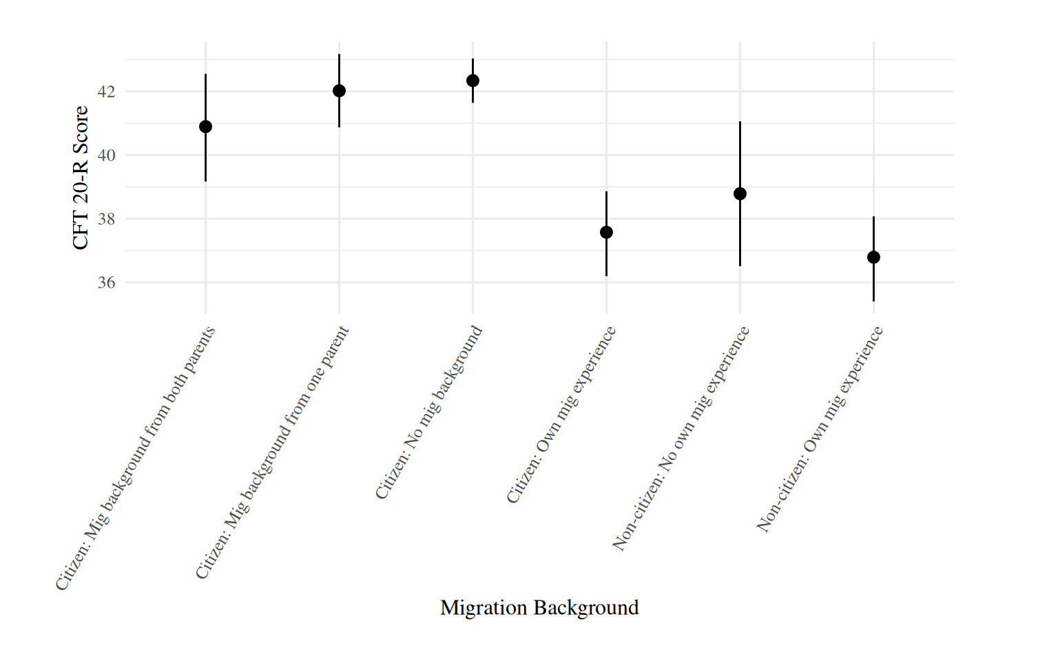
Less variation among migration categories.
3.2.6 Plots of the conditional age splines
distinct_tl <- tl_no_1st_twins %>%
  select(age, educ, mig, male) %>%
  mutate(male = FALSE, mig = "Citizen: No mig background") %>%
  distinct()

fitted_tl <- fitted(brm_age_by_educ, newdata = distinct_tl, summary = T, ndraws = 1000, probs = c(0.20, 0.80)) %>% as_tibble() %>%
  bind_cols(distinct_tl) %>%
  mutate(
    school_type = case_when(
      str_detect(educ, "ST") ~ educ,
      TRUE ~ NA_character_
    ),
    school_type = str_replace(school_type, "^[^ ]* ", ""),
    isced = case_when(
      str_detect(educ, "ST") ~ NA_character_,
      TRUE ~ educ
    ),
    isced = str_replace(isced, "^[^ ]* ", "")
  )

fitted_ST <- fitted_tl %>%
  filter(!is.na(school_type) & age <= 18)

fitted_ISCED <- fitted_tl %>%
  filter(!is.na(isced) & (age >= 19 & age <= 65) & !(age <= 21 & isced == "5a: Tertiary, e.g., college"))


max_age_per_ST <- fitted_ST %>%
                     group_by(school_type) %>%
                     summarise(max_age = max(age, na.rm = TRUE))


labels <- fitted_ST %>%
                inner_join(max_age_per_ST, by = "school_type") %>%
                filter(age == max_age)


# colour palette from https://jacksonlab.agronomy.wisc.edu/2016/05/23/15-level-colorblind-friendly-palette/
ggplot(data = fitted_ST, aes(x = age, y = Estimate, ymin = Q20, ymax = Q80, color = school_type, fill = school_type)) +
  scale_x_continuous(breaks = seq(12, 18, by = 2),
                   expand = expansion(add = c(0, 2))) +
  geom_line(linewidth = 1) +
  geom_ribbon(alpha = 0.2, linewidth = .01) +
  labs(x = "Age", y = "CFT 20-R Score", colour = "School Type") +
  geom_text_repel(data = labels %>% arrange(school_type),
    aes(label = c(school_type[1:5], "", school_type[7])), family = "Times", seed = 810, xlim = c(18.3, 20)) +
  geom_text_repel(data = labels %>% arrange(school_type),
    aes(label = c("", "", "", "", "", school_type[6], "")), family = "Times", nudge_x = 1.2, seed = 810) +
                       # Und bist du erst mein ehlich Weib,
                       # Dann bist du zu beneiden,
                       # Dann lebst du in lauter Zeitvertreib,
                       # In lauter Pläsier und Freuden.

                       # Und wenn du schiltst und wenn du tobst,
                       # Ich werd es geduldig leiden;
                       # Doch wenn du mein ggplot nicht lobst,
                       # Laß ich mich von dir scheiden.
  theme(
    panel.grid.major.y = element_blank(),
    panel.grid.minor.y = element_blank(),
    panel.grid.major.x = element_line(linetype = "dashed", size = 0.3),
    panel.grid.minor.x = element_blank(),
    legend.position = "none"
  ) +
  scale_color_manual(values = c("#009292","#000000","#ff6db6","#006ddb","#920000", "#490092","#6db6ff")) +
  scale_fill_manual(values = c("#009292","#000000","#ff6db6","#006ddb","#920000", "#490092","#6db6ff"))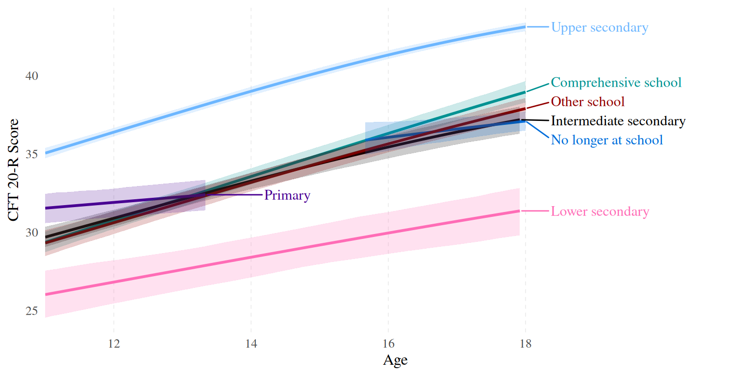
max_age_per_isced <- fitted_ISCED %>%
                     group_by(isced) %>%
                     summarise(max_age = max(age, na.rm = TRUE))


labels <- fitted_ISCED %>%
                inner_join(max_age_per_isced, by = "isced") %>%
                filter(age == max_age)

ggplot(data = fitted_ISCED, aes(x = age, y = Estimate, ymin = Q20, ymax = Q80, color = isced, fill = isced)) +
  scale_x_continuous(breaks = seq(19, 65, by = 9),
                     expand = expansion(add = c(1, 21)))  +
  geom_line(linewidth = 1) +
  geom_ribbon(alpha = .3, linewidth = .5) +
  labs(x = "Age", y = "CFT 20-R Score", colour = "ISCED 1997 Code")  +
  geom_text_repel(data = labels %>%
           arrange(isced),
    aes(label = isced), family = "Times", seed = 810, xlim = c(65, 100)) +
  theme(
    panel.grid.major.y = element_blank(),
    panel.grid.minor.y = element_blank(),
    panel.grid.major.x = element_line(linetype = "dashed", size = 0.3),
    panel.grid.minor.x = element_blank(),
    legend.position = "none"
  ) +
  scale_color_manual(values = c("#b66dff","#6db6ff","#009292", "#920000","#924900","#490092","#24ff24","#000000")) +
  scale_fill_manual(values = c("#b66dff","#6db6ff","#009292", "#920000","#924900","#490092","#24ff24","#000000"))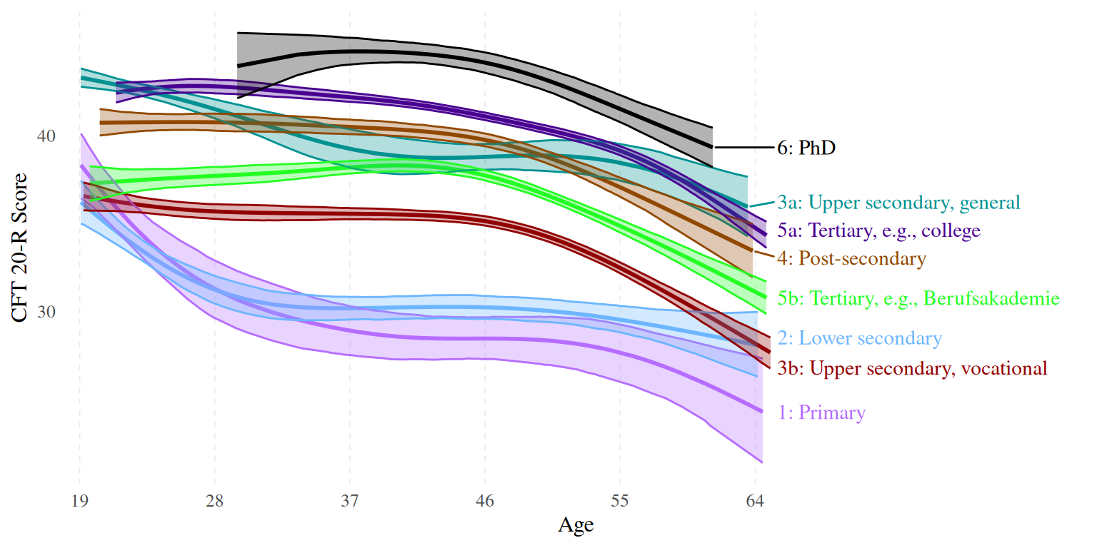
3.2.7 Sigma spline
plot(conditional_smooths(brm_age_by_educ), ask = FALSE, plot = FALSE)[[2]] 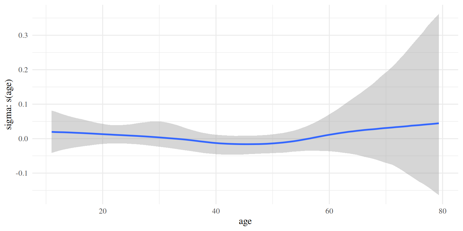
As expected, not much happening in the \(\sigma\) domain.
4 Poststratifcation
This is the P part of MRP.
4.1 Simulate a sample with the same joint distribution as the census
set.seed(810)
sim_pop_sample <- census %>%
  filter(age <= 65) %>%
  sample_n(size = 100000, # total census_n in the PS table is 6773812
           weight = census_n,
           replace = TRUE)
This code achieves this by creating a fake sample (N = 100000) in which the subgroup sample sizes are proportional to the sizes of the subgroups in the poststratification table. For example, if the subgroup consisting of the combination age = 12, male = TRUE, educ = Lower secondary, mig = Citizen: no migration background represents 0.2% of the total population (sum of the ns of all subgroups in the poststratification table census), then about 200 out of the 100,000 rows in sim_pop_sample will have this specific combination. replace was set to TRUE so that any given combination can be sampled more than once.
4.2 Estimate CFT 20-R for those simulated participants
Now that we have a post-stratified sample, we can use
tidybayes’s add_predicted_draws() function to draw
1000 samples (i.e., CFT 20-R Scores) from the posterior for each one of
the 10000 simulated participants in sim_pop_sample:
sim_pop_sample_with_draws <- sim_pop_sample %>%
  add_predicted_draws(brm_age_by_educ,
                      ndraws = 1000,
                      seed = 810,
                      allow_new_levels = TRUE) %>%
  mutate(.prediction = round(case_when(.prediction < 0 ~ 0,
                                 .prediction > 56 ~ 56,
                                 TRUE ~ .prediction)))

saveRDS(sim_pop_sample_with_draws, "data/simulated/sim_pop_sample_with_draws.rds")

# alternatively, import the version simulated using the brm we ran on the actual TL data
# sim_pop_sample_with_draws <- read_rds("data/simulated/sim_pop_sample_with_draws.rds")
This yields a dataframe in long format with 100000 (number of
simulated participants) * 1000 (number of draws from the posterior) =
100 million rows. allow_new_levels = TRUE is necessary for
estimating the outcome for combinations of the 4 predictors which do not
occur in the actual TL sample. This is inevitable in detailed enough
poststratification tables and was the case here as the
poststratification table we used had 6528 subcategories/rows. It wasn’t
the product of the number of categories of the four predictors \(69*2*15*6\) because a lot of combinations
of the variables were impossible, e.g., a PhD at the age of 11. The
mutate() call serves to set all predicted CFT 20-R 20-R
score scores which go below or above the scale limits (0 and 56,
respectively), to those scale limits.
5 Produce norms
5.1 Age group means and SDs
Here we aggregate the intelligence scores by age and compute the MRP corrected means and SDs (+ their SEs) for each age group:
means_sds_and_ses_MRP <- sim_pop_sample_with_draws %>%
  group_by(age, .draw) %>%
  summarise(mean_prediction = mean(.prediction),
            sd_prediction = sd(.prediction)) %>%
  group_by(age) %>%
  summarise(MRP_mean = mean(mean_prediction),
            MRP_se_of_mean = sd(mean_prediction),
            MRP_sd = sqrt(mean(sd_prediction^2)),
            MRP_se_of_sd = sd(sd_prediction))
means_sds_and_ses_MRP %>% head(14) %>% kable(digits = 2) %>% kable_styling(full_width = FALSE)| age | MRP_mean | MRP_se_of_mean | MRP_sd | MRP_se_of_sd |
|---|---|---|---|---|
| 11 | 31.38 | 0.32 | 7.74 | 0.22 |
| 12 | 32.13 | 0.30 | 7.88 | 0.23 |
| 13 | 33.40 | 0.30 | 7.99 | 0.24 |
| 14 | 34.56 | 0.30 | 8.04 | 0.23 |
| 15 | 35.47 | 0.34 | 8.13 | 0.23 |
| 16 | 36.75 | 0.32 | 8.01 | 0.22 |
| 17 | 38.42 | 0.29 | 7.88 | 0.19 |
| 18 | 39.09 | 0.34 | 7.79 | 0.22 |
| 19 | 38.05 | 0.87 | 8.15 | 0.30 |
| 20 | 38.95 | 0.47 | 8.08 | 0.26 |
| 21 | 38.87 | 0.35 | 8.07 | 0.23 |
| 22 | 38.61 | 0.30 | 8.06 | 0.19 |
| 23 | 38.26 | 0.29 | 8.11 | 0.19 |
| 24 | 38.12 | 0.28 | 8.05 | 0.20 |
This code chunk first aggregates by age and posterior draw (1000) to compute the mean and SD of CFT 20-R estimates across the 100000 simulated participants. Then it computes the means and SDs across the draws (which form the MRP means and SDs for each age group) and the SDs of the means and SDs calculated in the previous step, hence yielding the Bayesian SEs of the MRP means and SDs, respectively. Et voilà, an MRP corrected norm means and SDs! Here the 14 first rows are shown.
5.2 Age norm tables
5.2.1 Linearly transformed IQs
Here we calculate linearly transformed IQs for all cft scores that occur in the poststratified sample.
iq <- function(cft_score, mean, sd) {
  iq_score <- ((cft_score - mean) / sd) * 15 + 100
  return(iq_score)
}

iqs_linear <- sim_pop_sample_with_draws %>%
  filter(age <= 65) %>%
  left_join(select(means_sds_and_ses_MRP, c(MRP_mean, MRP_sd, age)), by = "age") %>%
  group_by(age, raw_score = .prediction) %>%
  summarise(MRP_IQ_linear = round(mean(iq(raw_score, MRP_mean, MRP_sd))))

iqs_linear %>% head(14) %>% kable %>% kable_styling(full_width = FALSE)| age | raw_score | MRP_IQ_linear |
|---|---|---|
| 11 | 0 | 39 |
| 11 | 1 | 41 |
| 11 | 2 | 43 |
| 11 | 3 | 45 |
| 11 | 4 | 47 |
| 11 | 5 | 49 |
| 11 | 6 | 51 |
| 11 | 7 | 53 |
| 11 | 8 | 55 |
| 11 | 9 | 57 |
| 11 | 10 | 59 |
| 11 | 11 | 61 |
| 11 | 12 | 62 |
| 11 | 13 | 64 |
5.2.2 Normalised (area transformed / normal rank transformed) IQs
Here we calculate normal rank transformed IQs for all cft scores that occur in the poststratified sample.
iqs_normalised <- sim_pop_sample_with_draws  %>%
  filter(age <= 65) %>%
  rename(raw_score = .prediction) %>%
  group_by(age, .draw) %>%
  mutate(n = n(),
         normal_transformed_score = qnorm((rank(raw_score) - 0.5) / n)) %>%
  mutate(iq_score = normal_transformed_score * 15 + 100) %>%
  group_by(age, raw_score) %>%
  summarise(MRP_IQ_normalised = round(mean(iq_score)))

iqs_normalised %>% head(14) %>% kable %>% kable_styling(full_width = FALSE)| age | raw_score | MRP_IQ_normalised |
|---|---|---|
| 11 | 0 | 50 |
| 11 | 1 | 51 |
| 11 | 2 | 51 |
| 11 | 3 | 51 |
| 11 | 4 | 53 |
| 11 | 5 | 54 |
| 11 | 6 | 55 |
| 11 | 7 | 56 |
| 11 | 8 | 58 |
| 11 | 9 | 60 |
| 11 | 10 | 61 |
| 11 | 11 | 63 |
| 11 | 12 | 64 |
| 11 | 13 | 66 |
6 Session info
sessionInfo()## R version 4.2.2 (2022-10-31)
## Platform: x86_64-pc-linux-gnu (64-bit)
## Running under: Rocky Linux 8.8 (Green Obsidian)
##
## Matrix products: default
## BLAS/LAPACK: /software/all/FlexiBLAS/3.2.1-GCC-12.2.0/lib64/libflexiblas.so.3.2
##
## locale:
## [1] LC_CTYPE=en_US.UTF-8 LC_NUMERIC=C
## [3] LC_TIME=en_US.UTF-8 LC_COLLATE=en_US.UTF-8
## [5] LC_MONETARY=en_US.UTF-8 LC_MESSAGES=en_US.UTF-8
## [7] LC_PAPER=en_US.UTF-8 LC_NAME=C
## [9] LC_ADDRESS=C LC_TELEPHONE=C
## [11] LC_MEASUREMENT=en_US.UTF-8 LC_IDENTIFICATION=C
##
## attached base packages:
## [1] stats graphics grDevices datasets utils methods base
##
## other attached packages:
## [1] bayesplot_1.10.0 marginaleffects_0.16.0 tidybayes_3.0.6
## [4] brms_2.20.4 Rcpp_1.0.11 kableExtra_1.3.4
## [7] ggrepel_0.9.4 forcats_1.0.0 stringr_1.5.1
## [10] dplyr_1.1.4 purrr_1.0.2 readr_2.1.4
## [13] tidyr_1.3.0 tibble_3.2.1 ggplot2_3.4.4
## [16] tidyverse_1.3.2
##
## loaded via a namespace (and not attached):
## [1] readxl_1.4.3 backports_1.4.1 systemfonts_1.0.5
## [4] plyr_1.8.9 igraph_1.5.1 splines_4.2.2
## [7] svUnit_1.0.6 crosstalk_1.2.1 rstantools_2.3.1.1
## [10] inline_0.3.19 digest_0.6.33 htmltools_0.5.7
## [13] fansi_1.0.5 magrittr_2.0.3 checkmate_2.3.0
## [16] googlesheets4_1.1.1 tzdb_0.4.0 modelr_0.1.11
## [19] RcppParallel_5.1.7 matrixStats_1.1.0 xts_0.13.1
## [22] svglite_2.1.2 timechange_0.2.0 prettyunits_1.2.0
## [25] colorspace_2.1-0 rvest_1.0.3 ggdist_3.3.0
## [28] haven_2.5.3 xfun_0.41 callr_3.7.3
## [31] crayon_1.5.2 jsonlite_1.8.7 zoo_1.8-12
## [34] glue_1.6.2 gtable_0.3.4 gargle_1.5.2
## [37] webshot_0.5.5 distributional_0.3.2 pkgbuild_1.4.2
## [40] rstan_2.32.3 abind_1.4-5 scales_1.2.1
## [43] mvtnorm_1.2-3 DBI_1.1.3 miniUI_0.1.1.1
## [46] viridisLite_0.4.2 xtable_1.8-4 stats4_4.2.2
## [49] StanHeaders_2.26.28 DT_0.30 collapse_2.0.6
## [52] htmlwidgets_1.6.3 httr_1.4.7 threejs_0.3.3
## [55] arrayhelpers_1.1-0 posterior_1.5.0 ellipsis_0.3.2
## [58] pkgconfig_2.0.3 loo_2.6.0 farver_2.1.1
## [61] sass_0.4.7 dbplyr_2.4.0 utf8_1.2.4
## [64] tidyselect_1.2.0 labeling_0.4.3 rlang_1.1.2
## [67] reshape2_1.4.4 later_1.3.1 munsell_0.5.0
## [70] cellranger_1.1.0 tools_4.2.2 cachem_1.0.8
## [73] cli_3.6.1 generics_0.1.3 broom_1.0.5
## [76] evaluate_0.23 fastmap_1.1.1 yaml_2.3.7
## [79] processx_3.8.2 knitr_1.45 fs_1.6.3
## [82] nlme_3.1-162 mime_0.12 xml2_1.3.5
## [85] compiler_4.2.2 shinythemes_1.2.0 rstudioapi_0.15.0
## [88] reprex_2.0.2 bslib_0.6.0 stringi_1.8.2
## [91] highr_0.10 ps_1.7.5 Brobdingnag_1.2-9
## [94] lattice_0.22-5 Matrix_1.5-3 markdown_1.11
## [97] shinyjs_2.1.0 tensorA_0.36.2 vctrs_0.6.4
## [100] pillar_1.9.0 lifecycle_1.0.4 jquerylib_0.1.4
## [103] bridgesampling_1.1-2 insight_0.19.6 data.table_1.14.8
## [106] httpuv_1.6.12 QuickJSR_1.0.8 R6_2.5.1
## [109] promises_1.2.1 renv_1.0.3 gridExtra_2.3
## [112] codetools_0.2-19 colourpicker_1.3.0 gtools_3.9.5
## [115] withr_2.5.2 shinystan_2.6.0 mgcv_1.8-42
## [118] parallel_4.2.2 hms_1.1.3 grid_4.2.2
## [121] coda_0.19-4 rmarkdown_2.25 cmdstanr_0.6.1
## [124] googledrive_2.1.1 shiny_1.8.0 lubridate_1.9.3
## [127] base64enc_0.1-3 dygraphs_1.1.1.6